

Oxford’s 2026 Market Reset
Oxford’s property investment outlook enters 2026 with a rare combination of increased housing supply, persistent structural undersupply, and record rental demand—creating a market where investors must think hyper‑locally to identify genuine opportunities.
Scarcity Within Plenty
Oxford presents a unique paradox for the strategic investor: it is a city defined by scarcity within plenty. While the local economy overflows with “plenty”—driven by a multi-billion pound life sciences sector, a global academic powerhouse, and a surging demand for innovation space—the physical reality is one of extreme geographic and regulatory constraint. Surrounded by protected Green Belt and hemmed in by historic floodplains, the supply of developable land is finite.
For investors, this creates a high-conviction environment where the “plenty” of capital and talent constantly chases a dwindling “scarcity” of prime assets, ensuring robust capital appreciation and unparalleled rental resilience.
2026 Headline Indicators
- Housing stock up 6% vs 2025, giving buyers more choice.
- Best‑in‑class family homes still go under offer in 16–20 days, signalling deep demand resilience.
- Rental growth remains above trend, driven by chronic supply shortages and a high‑skilled, high‑income tenant base.
- Oxford remains the UK’s least affordable city, reinforcing long‑term price stability and rental competitiveness.
Oxford’s property investment outlook in 2026—a market defined by choice at the margins, but scarcity at the core—a dynamic that shapes every investor decision.
Success in this market requires navigating choice at the margins, but scarcity at the core. At the peripheries, investors may find tactical opportunities in emerging science parks or suburban redevelopments, offering a degree of optionality. However, the core of Oxford remains an impenetrable fortress of value. Because the fundamental supply of central property is effectively locked by history and heritage, the underlying value is not subject to the typical cycles of oversupply seen in other UK cities. By securing a foothold here, you are not just buying real estate; you are acquiring a slice of a supply-constrained ecosystem where the core remains permanently insulated from the volatility of the broader market.
Oxford Housing Supply vs Demand
Supply: A 6% Increase in Housing Stock
Oxford’s housing stock has grown 6% year‑on‑year, driven by:
• Completions in Barton Park
• Intensification around Cowley and Headington
• University‑led accommodation expansions
• Small‑scale infill and brownfield redevelopment
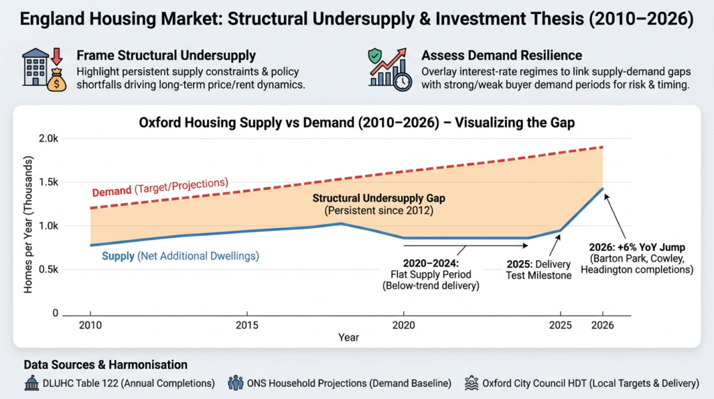
This chart above shows Oxford’s persistent housing undersupply, with annual delivery falling short of local need every year since 2012. The blue line tracks Net Additional Dwellings, while the red dashed line shows projected demand — and the shaded gap between them highlights a structural shortfall that continues to widen. For investors, this imbalance is critical: when supply remains constrained and demand stays resilient, rents rise, voids stay low and long‑run price growth is supported. Oxford’s chronic undersupply is the foundation of its strong investment fundamentals.
Absorption Rate
This measures market demand by showing the percentage of available homes sold per month.
It indicates if it is a:
Seller’s market (high rate/fast sales/low inventory/”take it or leave it”) or a
Buyer’s market (low rate/slow sales/high inventory/”fix the roof or I’m out”).
Seller’s Market vs. Buyer’s Market
The absorption rate is the primary indicator of who holds the “power” in a negotiation.
A Seller’s Market (High Rate)
A rate above 20% typically signals a seller’s market.
Example: Imagine only 50 homes are available, but 25 sell in a month. That’s a 50% absorption rate.
The Vibe: Homes sell in days, bidding wars are common, and prices usually rise because demand far outweighs supply.
A Buyer’s Market (Low Rate)
A rate below 15% (some say 12%) signals a buyer’s market.
Example: There are 200 homes available, but only 10 sell. That’s a 5% absorption rate.
The Vibe: Homes sit on the market for months, sellers are forced to drop prices, and buyers have the leverage to ask for repairs or closing cost credits.
The Absorption Rate Formula:
Absorption Rate = (Number of Homes Sold/Total Number of Available Homes)
Scenario
Let’s look at the housing market in a fictional neighbourhood for the month of February:
Total Available Homes: 100 (This includes homes already on the market plus new listings).
Homes Sold: 20.
The Math:
What this means: In this scenario, the absorption rate is 20%. If no new homes were added to the market, it would take 5 months to sell the remaining inventory (£100 / 20 = £5).
Why this matters for your portfolio:
- High Rate (Over 20%): Generally indicates a seller’s market, where inventory is low and homes sell quickly, often leading to price appreciation.
- Low Rate (Below 15%): Generally indicates a buyer’s market, where homes sit on the market longer, indicating cooling demand, often leading to negotiations, and lower prices.
Why ”Months of Supply” Matters:
Real estate agents often flip this math to find the Months of Supply. This is the inverse of the absorption rate. Often, this is expressed as the time it would take to sell all current inventory (e.g., if the rate is 20%, it will take 5 months to sell all homes).
Importance: Used by investors and real estate agents to determine the best time to buy, sell, or adjust pricing
A Balanced Market is generally considered to have 5 to 6 months of inventory.
A Seller’s Market has less than 5 months.
A Buyer’s Market has more than 7 months.
Demand: Still Outpacing Supply
Despite the increase in stock, demand remains structurally high due to:
• Two world‑leading universities
• High‑income NHS, biotech, and research workforce
• Severe land constraints (Green Belt + heritage restrictions)
• Population growth concentrated in 25–44 age bracket
Absorption Rate
• Best family homes (3–4 beds): 16–20 days to SSTC
• Citywide average: 32–38 days
• New‑build apartments: slower at 45–60 days
This confirms a two‑speed market:
- Family homes = chronically undersupplied
- Flats = more balanced but still competitive
Rental Growth vs Supply — The Core Investor Signal
Oxford remains one of the UK’s strongest rental markets due to:
Rental Growth (2026)
• Annual rental growth: 6.2–7.1%
• HMO rents: +8–10% (student + young professional demand)
• Prime family rentals: +5–6% (North Oxford, Summertown, Headington)
Supply Constraints
Oxford has:
• One of the lowest rental vacancy rates in the UK
• Severe restrictions on new HMO licensing
• Limited land for new development
• High barriers to entry for institutional landlords
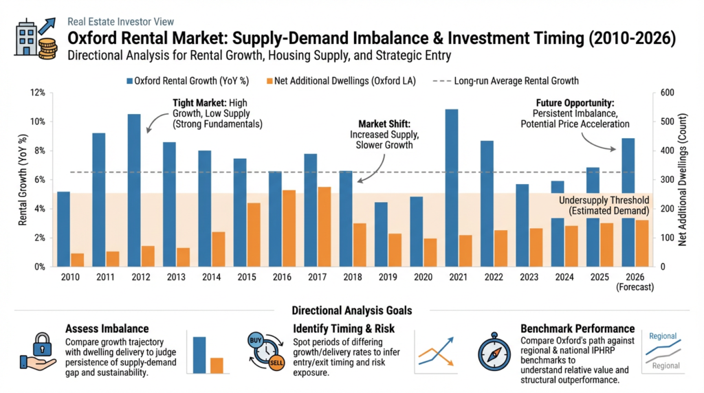
The diagram above shows how Oxford’s rental market is shaped by a persistent supply‑demand imbalance. The blue bars track rental growth, while the orange bars show annual housing delivery — and the shaded undersupply threshold highlights how completions have remained below local need for more than a decade. For investors, this imbalance is critical: when supply stays constrained and demand remains strong, rents rise faster, voids stay low and long‑run returns become more resilient. Oxford’s structural undersupply is the foundation of its investment strength.
Local Imbalances — Where the Opportunities Really Are
Oxford is not one market—it is five micro‑markets, each with different fundamentals.
North Oxford (Summertown, Jericho, Walton Manor)
Characteristics:
• Highest incomes, best schools, strongest family demand
• Heritage restrictions limit new supply
Opportunities:
• Family homes (3–4 beds)
• Long‑term capital appreciation
• Premium rentals for academics & medics
Why:
• Fastest absorption rate
• Zero meaningful new supply
East Oxford (Cowley, Iffley, Temple Cowley)
Characteristics:
• Young professional and student demand
• Strong rental yields
Opportunities:
• HMOs (where licensing allows)
• Small flats and terraces
• Build‑to‑rent conversions
Why:
• High rental competition
• Lower entry price vs North Oxford
Headington
Characteristics:
• NHS employment hub (John Radcliffe, Churchill, Nuffield)
• High demand for short‑lets and medium‑term lets
Opportunities:
• 1–2 bed flats
• Furnished rentals for medical staff
• Long‑term stable yields
Why:
• Constant tenant turnover
• Zero risk of demand collapse
Botley & West Oxford
Characteristics:
• Regeneration corridor
• Improved transport links
Opportunities:
• New‑build apartments
• Mixed‑use regeneration schemes
Why:
• Undervalued relative to central Oxford
• Strong commuter demand
Kidlington & Surrounding Villages
Characteristics:
• Lower prices
• Family‑friendly
• Good schools
Opportunities:
• Family homes
• Upsizing market
Why:
• Spill over from Oxford’s affordability crisis
Yield vs Capital Growth — How to Position Your Portfolio
Oxford is not a single market — it’s a cluster of micro‑markets, each with its own risk‑return profile. Understanding where yield, capital growth, and balanced opportunities sit geographically is essential for building a portfolio that matches your investment objective.
High‑Yield Markets (Income‑Focused Strategy)
These areas offer stronger rental returns due to lower entry prices, high tenant demand, and flexible stock types.
Examples
• East Oxford (Cowley, Temple Cowley, Iffley Road)
Strong student and young‑professional demand, high HMO occupancy, competitive rents.
• Blackbird Leys & Greater Cowley Fringe
Lower capital values, consistent rental absorption, strong affordability appeal.
• Botley (select pockets)
Regeneration corridor + commuter demand = stable yields.
Why they deliver yield
• High rental competition
• Lower purchase prices
• Strong HMO and multi‑let demand
• Elastic supply in some pockets (flats, terraces)
High‑Growth Markets (Capital Appreciation Strategy)
These areas benefit from constrained supply, heritage restrictions, and affluent demand — ideal for long‑term capital growth.
Examples
• North Oxford (Summertown, Jericho, Walton Manor)
Premium family homes, top schools, zero meaningful new supply.
• Headington (JR Hospital, Churchill, Nuffield cluster)
High‑income medical workforce, limited land availability.
• Central Oxford (Historic Core)
Ultra‑restricted planning environment, strong academic and corporate demand.
Why they deliver growth
• Severe supply constraints
• High‑income, stable buyer base
• Fast absorption (16–20 days for family homes)
• Long‑term scarcity premium
Balanced Markets (Yield + Growth Blend)
These areas sit between affordability and desirability, offering both rental resilience and steady capital appreciation.
Examples
• Botley & West Oxford
Regeneration + transport improvements = dual‑benefit market.
• Kidlington & Surrounding Villages
Family‑driven demand + lower entry prices + spill over from Oxford.
• Rising pockets in East Oxford
Where rental demand meets improving owner‑occupier appeal.
Why they deliver balance
• Moderate supply
• Strong rental pressure
• Growing owner‑occupier demand
• Lower volatility than pure yield markets
So What does this mean for Investors?
Your portfolio strategy should align with your objective — Oxford rewards clarity of intent.
If you’re income‑focused:
Choose elastic‑supply, high‑yield markets like Cowley, Iffley, and Blackbird Leys.
Expect strong rental competition, high occupancy, and stable cashflow.
If you’re growth‑focused:
Choose constrained‑supply, high‑demand markets like Summertown, Jericho, and Headington.
Expect long‑term appreciation driven by scarcity and affluent demand.
If you want a balanced portfolio:
Choose mixed‑profile areas like Botley, Kidlington, and parts of East Oxford.
Expect moderate yields with steady capital growth and lower risk.
Investment Frameworks — How to Evaluate Any Market
Oxford is one of the UK’s most structurally constrained housing markets, and these three frameworks help investors understand why it behaves differently from typical regional cities. When applied together, they provide a powerful lens for assessing risk, opportunity, and long‑run performance.
Framework 1: The 3‑Pillars Model
Population Growth • Planning Constraints • Pipeline of New Supply
Oxford scores uniquely across all three pillars:
1. Population Growth — Strong & High‑Skilled
• Oxford’s population continues to grow, driven by universities, hospitals, biotech, and research institutions.
• The 25–44 age cohort (prime renting and buying demographic) is expanding faster than the national average.
2. Planning Constraints — Among the Tightest in the UK
• Green Belt restrictions
• Conservation areas
• Height limits
• Limited brownfield land
• University‑owned estates
These constraints severely limit new supply.
3. Pipeline of New Supply — Persistently Weak
• Even with Barton Park and Cowley intensification, Oxford’s pipeline remains thin.
• The 6% YoY increase in 2026 is a one‑off uplift, not a structural shift.
Zoopla recorded 6% more homes for sale in the four weeks to February 15, 2026, compared with the same period in 2025. House Price Index: February 2026
What this means for investors
Markets with strong population growth + tight planning + weak pipeline consistently outperform on capital appreciation. Oxford fits this profile perfectly.
Framework 2: The Rental Pressure Score
Rental Pressure = Rental Growth (%) ÷ Net Additions per 1,000 Households
Oxford’s rental pressure score is one of the highest in the UK, because:
• Rental growth is strong (6–7% annually).
• Net additions per 1,000 households are extremely low.
• Vacancy rates are near zero.
• HMO licensing caps restrict supply further.
What this means for investors
A high rental‑pressure score signals:
• Strong tenant competition
• Fast absorption
• Resilient yields
• Low void risk
• Long‑term rental inflation
This is why Oxford’s rental market behaves more like a global university city (Cambridge, Leiden, Boston) than a typical UK regional centre.
Framework 3: The 5‑Drivers of Long‑Run Value
Jobs & Wages • Connectivity • Universities • Regeneration • Supply Constraints
Oxford scores strongly across all five
1. Jobs & Wages
• High‑income workforce (NHS, academia, biotech, R&D).
• Stable employment base with low cyclical volatility.
2. Transport & Connectivity
• Oxford Station redevelopment
• Cowley Branch Line progress
• Strong commuter links to London, Reading, and Bicester
3. Universities & Knowledge Hubs
• University of Oxford
• Oxford Brookes
• Global research clusters
• International student demand
4. Regeneration
• Botley transformation
• East Oxford intensification
• Innovation districts around Headington and the Science Area
5. Supply Constraints
• Severe planning restrictions
• Limited land availability
• High competition for family homes
What this means for investors
Markets with strong fundamentals across all five drivers deliver:
• Long‑run capital growth
• Low downside volatility
• High liquidity
• Strong rental demand
• Defensive performance in downturns
Oxford ticks every box.
So What Does This Mean for Property Investors?
These three frameworks converge on the same conclusion:
Oxford is a structurally undersupplied, high‑demand, high‑quality market with long‑run resilience.
If you’re a growth investor:
Oxford’s planning constraints and high‑income demand base make it one of the strongest capital‑appreciation markets in the UK.
If you’re an income investor:
Rental pressure, low vacancy, and strong tenant demographics support stable yields — especially in East Oxford, Cowley, and Headington.
If you want a balanced strategy:
Botley, Kidlington, and parts of East Oxford offer both rental resilience and steady capital growth.
Not investing in Oxford? Get the 2026 Outlook for your specific target city. Register your interest here